Results
Descriptive Statistics: Total sample
Ethnicity
The distribution of ethnicity for all offenders in the sample is shown in Figure 1. Ethnicity information was collected from the IOM computer system and confirmed during interview. The distribution indicated that overall the YOU’s reflected the ethnicity distribution found in mainstream prison units.
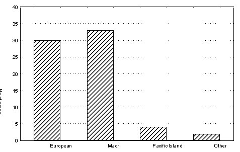
Figure 1: Distribution of ethnicity in total sample
However, when ethnicity was examined across the three YOU’s, marked differences in distribution were found. Table 1 shows that while the Hawkes Bay unit had a virtually even split between Maori and European, the WBOP unit were 71% Maori and the Christchurch unit 68% European. This difference in ethnicity distribution was found using Pearson Chi Square analysis to be statistically significant (X? = 16.57, df = 6, p = .011). No significant difference was found based on ethnicity for any of the offence variables or risk measures used in this study.
|
Ethnicity |
Hawkes Bay (N = 23) |
WBOP (N = 21) |
Christchurch (N = 25) |
|
European |
39% |
19% |
68% |
|
Maori |
43% |
71% |
32% |
|
Pacific Island |
9% |
10% |
0% |
|
Other |
9% |
0% |
0% |
Age variables
Age of first conviction. The mean age at which youth offenders in the study were first convicted in either Youth Court or District Court was found to be M = 15.62 (SD = 1.26). The range in age was from 13 years of age through to 18. The distribution in age of first conviction is shown below in Figure 2.
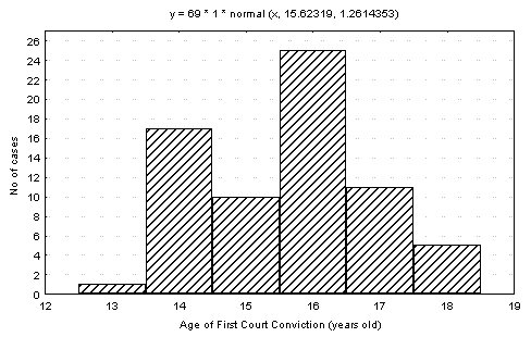
Figure 2: Distribution of age of first conviction for all study participants
of age (see Table 2). No significant difference was found for age of first conviction between Very few were convicted in court before 15 years of age (26%) with half the sample convicted at either 15 or 16 years the three YOU in the study.
|
Age (Years) |
Percentage |
|
13 |
1% |
|
14 |
25% |
|
15 |
15% |
|
16 |
36% |
|
17 |
16% |
|
18 |
7% |
Table 2: Percentage by age of conviction for total sample
Current age. The mean current age for the sample was found to be M = 17.5 (SD .76) with a range of 16-19. When the age distribution was graphed in Figure 3 it is clear the only a very small number of youth offenders incarcerated in the YOU’s were either 16 or 19 years of age. In total 84% were 17 or 18 years of age when assessed. A significant difference was found between the three YOU’s in the study for current age. A one way ANOVA using age and YOU placement found that the WBOP unit mean age (16.95) was significantly lower than the other two units (F = 11.17, df = 2 , p = 0.0000). The interaction between the three unit mean current offender ages is shown in Figure 4 on the next page.
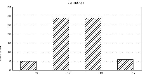
Figure 3: Distribution of current age of study participants
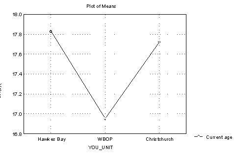
Figure 4: Interaction between mean age and YOU placement
Index and previous offending
Index offending. In looking at the offending that had resulted in the longest current sentence Figure 5 shows the distribution of index offending for the total sample. Aggravated robbery was the most frequent imprisonment offence followed by dishonesty (mainly burglary but also included theft ex car and stealing motor vehicles) and serious assault (aggravated wounding, assault with intent to injure, GBH). Note that in classifying sexual offences those in which there was rape of a victim over 12 years were listed as rape but those involving victims under 12 were listed as Child Sex Offences (CSO) due to the larger age difference between the offender and victim(s).
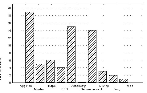
Figure 5: Distribution of index offending for youth offenders in the study
If the distribution of index offences was reclassified on the basis of serious violent/sexual, offending and other, then 70% of the sample had violent/sexual offences with the majority having violent (55%). When index offence distribution was examined using Chi Square analysis no significant differences in offence distribution were found between the three units (see Appendix C graphs). However, all had a number of violent offenders, typically for Aggravated Robbery, with WBOP having the largest number of murder type offences. The Hawkes Bay unit had no offenders convicted of sexual offences while the Christchurch unit was found to have the largest percentage with 26% convicted of rape and CSO. Details on the differences in index offence distribution are contained in Table 3.
|
Index offence type |
Hawkes Bay |
WBOP |
CHCH |
|
Aggravated Robbery |
30% |
19% |
32% |
|
Murder |
4% |
19% |
0% |
|
Rape |
0% |
5% |
20% |
|
CSO |
0% |
14% |
4% |
|
Dishonesty |
30% |
19% |
16% |
|
Serious assault |
26% |
19% |
16% |
|
Driving |
4% |
0% |
8% |
|
Drug |
0% |
5% |
4% |
|
Misc |
4% |
0% |
0% |
Descriptive analysis of offence related variables. In addition to index offending data were gathered on a number of other offence related variables. These were sentence length (calculated in months), total number of convictions, including their index offence(s), criminal versatility (number of difference offence types based on 11 categories), and number of violent and sexual offences. Details on the means and range for these variables are contained below in Table 4.
|
Variables |
N |
Mean |
Min |
Max |
Std.Dev. |
|
Sentence length |
69 |
32.08 |
3 |
120 |
25.19 |
|
Total convictions |
69 |
16.92 |
1 |
80 |
17.05 |
|
Criminal versatility |
69 |
4.17 |
1 |
11 |
2.19 |
|
Violent convictions |
69 |
2.20 |
0 |
12 |
2.23 |
|
Sexual convictions |
69 |
0.43 |
0 |
11 |
1.62 |
Table 4 reveals that the offenders in the YOU’s typically were sentenced to approximately 2 years 8 months. This means that in the main they are sentenced under the Sentencing Act 2002 and eligible for parole after a third of their sentence. In the case of the mean sentence length this means possible parole after 11 months. The youth offenders had a mean total number of convictions of 17 including their index offences and these offences were in a mean of four difference offence types. The mean number of violent convictions at 2.20 is high when not all were convicted of violence with a far lower mean for total convictions for sexual offending, a low base rate offence type.
Multivariate analysis of offence variables by YOU. When the variables listed in Table 4 were examined using a one way ANOVA where the grouping variable was the three YOU’s significant differences were found for mean total convictions and criminal versatility.
|
Analysis of Variance (maindata.sta) |
|
|
|
|
|
|||
|
Marked effects are significant at p < .05000 |
|
|
|
|
|
|||
|
|
SS |
df |
MS |
SS |
Df |
MS |
|
|
|
|
Effect |
Effect |
Effect |
Error |
Error |
Error |
F |
P |
|
Sentence length |
3183 |
2 |
1591.94 |
39973.5 |
66 |
605.66 |
2.62 |
0.0797 |
|
Total convictions |
1804 |
2 |
902.21 |
17966.2 |
66 |
272.21 |
3.31 |
0.0424 |
|
Criminal versatility |
45.08 |
2 |
22.54 |
282.82 |
66 |
4.28 |
5.26 |
0.0075 |
|
Total violence con |
18.08 |
2 |
9.04 |
321.07 |
66 |
4.86 |
1.85 |
0.1638 |
|
Total sex convict |
6.52 |
2 |
3.26 |
172.43 |
66 |
2.61 |
1.24 |
0.2937 |
Table 5: ANOVA results for risk variables with YOU placement as the grouping variable
The interactions between the YOU placement and the means for the significant variables are shown in the graphs on the next page. Figure 6 clearly reveals that the mean total convictions for the Hawkes Bay (M = 21) and Christchurch (M = 20) YOU’s were significantly higher then the WBOP unit (M = 9).
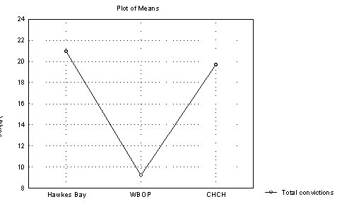
Figure 6: ANOVA Interaction between total convictions and YOU placement
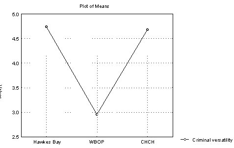
Figure 7: ANOVA Interaction between mean criminal versatility and YOU placement
Figure 7 clearly reveals that the mean number of offence types indicated by the variable criminal versatility were significantly higher for the Hawkes Bay and Christchurch (M = 5) YOU’s than the WBOP unit (M = 3). Both total number of previous convictions and criminal versatility are associated with a higher risk of reoffending.
Descriptive statistics on the four risk measures
Data for the PCL: YV, YLS/CMI, and RSYO was gathered for all 69 study participants, and RoC*RoI for 66. Details on the means, standard deviations, and score range are listed below in Table 6 for the total scores for the four measures and subscales.
|
Risk Measures |
Valid N |
Mean |
Min |
Max |
SD |
|
RoC*RoI |
66 |
0.58 |
0.09 |
0.89 |
0.17 |
|
PCL: YV |
69 |
25.09 |
9 |
39 |
7.29 |
|
F1 Interpersonal |
69 |
4.04 |
1 |
8 |
1.97 |
|
F2 Affective |
69 |
5.43 |
1 |
8 |
1.90 |
|
F3 Behaviour |
69 |
7.13 |
1 |
10 |
2.20 |
|
F4 Antisocial |
69 |
5.62 |
1 |
10 |
2.40 |
|
RSYO |
69 |
38.48 |
9 |
62 |
12.97 |
|
Disruptive ages 4-10 (S2) |
69 |
10.44 |
0 |
24 |
7.07 |
|
Delinquent ages 7-14 (S3) |
69 |
14.21 |
2 |
24 |
5.08 |
|
Adolescent offending 10-18 (S4) |
69 |
13.81 |
3 |
21 |
3.80 |
|
YLS/CMI |
69 |
23.49 |
5 |
35 |
6.38 |
|
Offences |
69 |
2.19 |
0 |
5 |
1.56 |
|
Family |
69 |
2.72 |
0 |
6 |
1.72 |
|
Education/Employ |
69 |
4.25 |
0 |
7 |
1.45 |
|
Peers |
69 |
3.32 |
0 |
4 |
0.96 |
|
Substance abuse |
69 |
3.22 |
0 |
5 |
1.41 |
|
Leisure |
69 |
1.19 |
0 |
3 |
0.93 |
|
Personality |
69 |
3.94 |
0 |
7 |
1.59 |
|
Attitude |
69 |
2.67 |
0 |
5 |
1.40 |
RoC*RoI. The mean for RoC*RoI at .58 is high compared to the general prison population (approximately .40). Figure 8 below reveals a normal distribution of RoC*RoI scores with a positive skew reflecting the high average risk of serious recidivism.
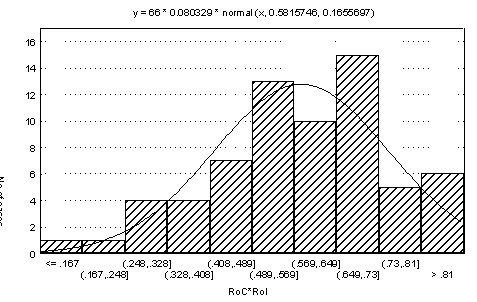
Figure 8: Distribution of RoC*RoI scores for the study sample
The RoC*RoI score distribution was divided up into risk categories, Low = 0-.49, Medium = .50-.69, and High = .70+ (see Table 7). This showed that 29% of the sample would meet the departmental classification as high risk offenders with 71% above the .50 cut-off for intervention (see Appendix D for a distribution graph of risk categories).
|
RoC*RoI risk category |
Percentage of sample |
|
Low 0-.49 |
29% |
|
Medium .50-.69 |
42% |
|
High .70 + |
29% |
PCL: YV. The mean for the PCL: YV (25.09) is similar to other studies using the instrument with incarcerated violent adolescent offenders (Forth, et al., 2003). The range was skewed high 9-39 again reflecting the high risk nature of this youth offender population. The distribution in Figure 9 on the next page indicates a number of the sample scoring 30 or more, the cut-off usually associated with severe interpersonal and affective deficits. The mean scores for the four factors contained in the PCL: YV are also high, especially for Factor 2 (M = 5.43): Affective and Factor 3 (M = 7.13), Behavioral. The distribution of all the factor scores is shown in Figure 10. While Factor 1 and 2 are associated with interpersonal and affective deficits and relate more to poor responsivity, the Factor 3 and 4 scores relate to a pattern of antisocial behaviour across settings and time.
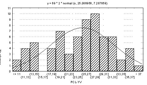
Figure 9: Distribution of PCL: YV scores for the study sample
When the PCL: YV scores are split into the risk categories used in the manual similar percentages were found for the three risk groups shown in Table 8 (See Appendix D for a distribution graph of risk categories).
|
PCL: YV risk category |
Percentage of sample |
|
Low < 20 |
22% |
|
Medium 20-29 |
51% |
|
High 30+ |
27% |
RYSO. The mean for the RYSO was also skewed high for this sample. Figure 11 below shows a normal distribution for the total score with some participants having very high scores on the risk instrument.
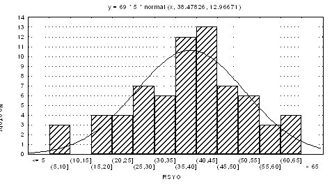
Figure 11: Distribution of RSYO scores for the study sample
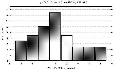
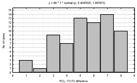
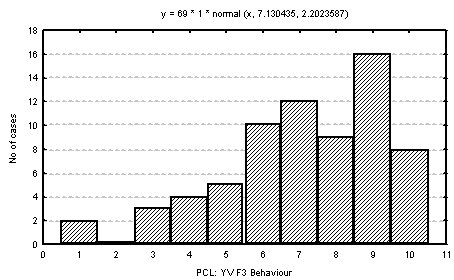
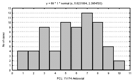
Figure 10: Distribution of scores for the PCL: YV four factors
The RSYO total score was divided into risk categories based on the probability of general reoffending (Low = < 35 [50% recidivism]; Medium = 35-55 [51-69% recidivism]; High = 56+ [70% = recidivism]). Table 9 shows the distribution of scores (see Appendix D for a distribution graph of risk categories).
|
RSYO risk category |
Percentage of sample |
|
Low < 35 |
33% |
|
Medium 35-55 |
57% |
|
High 56+ |
10% |